stsb3This is the homepage for structural time series, round 3. (Don't ask about 1 and 2.) You can get the library by visiting the project Gitlab.
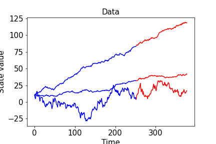
Here’s some data. The underlying generating process is a random walk.
t1 = 252
n = 3
n_pred = int(0.5 * t1)
loc = torch.randn((3, 1)) * 0.1
scale = torch.randn((3, 1)).exp()
data = 10.0 + (loc + scale * torch.randn((n, t1 + n_pred,))).cumsum(dim=-1)
train_data = data[:, :t1]
test_data = data[:, t1:]

for k in range(n):
    plt.plot(range(t1), train_data[k], color='blue')
plt.plot(range(t1, t1 + n_pred), test_data[k], color='red')In stsb3, expressing a random walk model is pretty easy.
dgp = stsb3.sts.RandomWalk(
    size=n,
    name="rw",
    t1=t1,
)
Under the hood, priors are automatically generated for you if you don’t specify them. We’ll get to that later. stsb3 is deeply integrated with torch and pyro. For example, we can introduce a data likelihood function that exposes a built-in fit method that wraps pyro’s variational inference and autoguide capabilities.
model = stsb3.sts.GaussianNoise(
    dgp,
    name="likelihood",
    data=train_data,
    size=n,
    scale=torch.tensor(0.1)
)
prior = model.prior_predictive(nsamples=100)
# you can pass through lots of arguments to pyro inference -- or not! -- more on that later
model.fit(method_kwargs=dict(niter=4000), verbosity=2e-3)
posterior = model.posterior_predictive(nsamples=100)

output$ On iteration 0, loss = 312638.2765661088
On iteration 500, loss = 8518.322829425453
On iteration 1000, loss = 4281.812141907593
On iteration 1500, loss = 3562.282855011227
On iteration 2000, loss = 2092.1784127041224
On iteration 2500, loss = 3279.810886447865
On iteration 3000, loss = 1533.6185196929034
On iteration 3500, loss = 703.8973624693259
After training, we can inspect the prior and posterior predictive empirical densities of what we’ve modeled as a latent random walk:
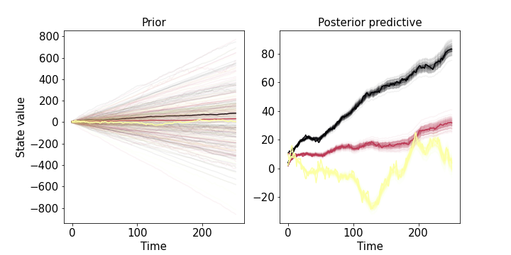
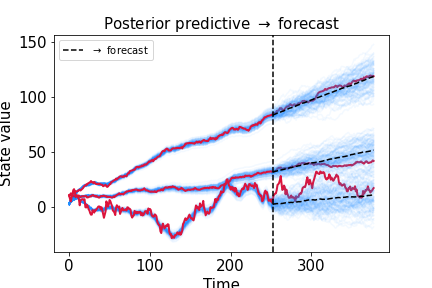
One of the objectives of stsb3 is to enable white-box time series modeling that still allows for performant forecasting. Let’s see how well we learned the model parameters as measured by forecast performance.
# forecast the latent state forward
posterior_forecast = stsb3.sts.forecast(
    dgp,
    posterior,
    Nt=n_pred,
    nsamples=100
)
Everything below is a valid stsb3 model.
# autoregressive model of order 1
ar1 = stsb3.sts.AR1(t1=t1, size=n, name="ar1")

# semi-local linear trend
latent_loc =  stsb3.sts.AR1(t1=t1, size=n, name="latent_loc")
sllt = stsb3.sts.RandomWalk(t1=t1, size=n, name="sllt", loc=latent_loc)

# seasonal global trend model
n_seasons = 7
s = stsb3.sts.DiscreteSeasonal(name="s", size=n, t1=t1, n_seasons=n_seasons,)
gt = stsb3.sts.GlobalTrend(t1=t1, size=n, name="global trend", beta=dist.Normal(0.05, 1e-2).expand((n,)))
sgt = s + gt + ar1

# stochastic volatility asset price
dt = torch.tensor(1.0 / t1)  # normalize to years
log_vol = stsb3.sts.CCSDE(t1=t1, size=n, dt=dt,
            loc=dist.Normal(0.0, 1.0).expand((n,)),
            ic=dist.Normal(0.0, 0.1).expand((n,)))
log_asset_price = stsb3.sts.CCSDE(t1=t1, size=n, dt=dt, scale=log_vol.exp())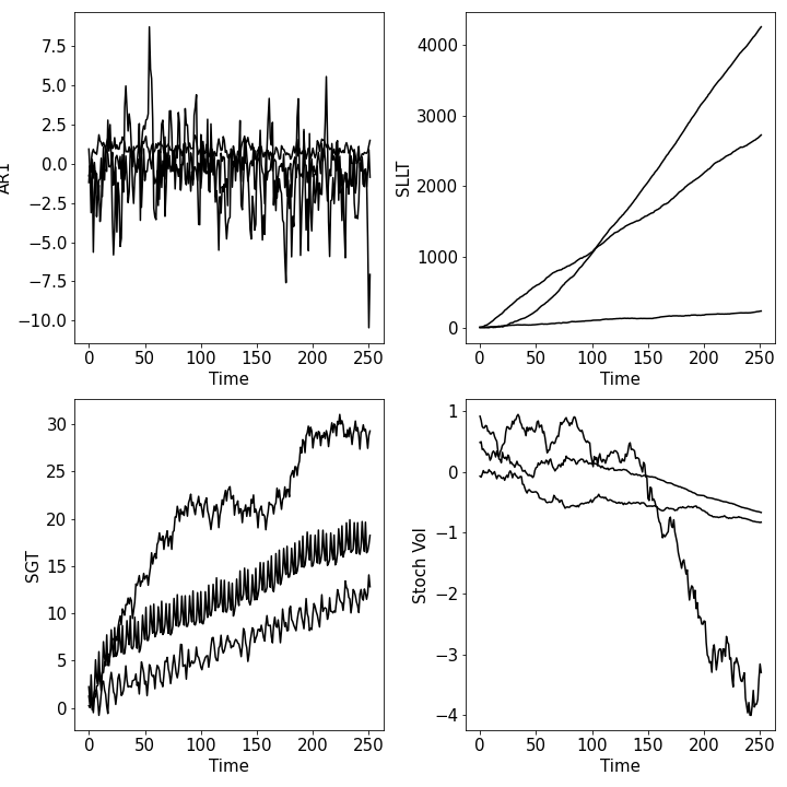
Every one of these models can be sampled from, as we do above, and can be confronted with data by wrapping it in an stsb3.sts.NoiseBlock instance, or by embedding the model within a more general pyro stochastic function (again more on that later). Underneath, stsb3 implements a context-sensitive model grammar that allows for arbitrary addition and composition of models as long as certain parameter space restrictions are met. (The grammar is detailed in a paper, if you care.) The point is that stsb3 allows you to easily construct expressive time series models that are always interpretable by definition.
Right now, the following primitive blocks are implemented:
AR1: autoregressive model of order 1CCSDE: constant-coefficient stochastic differential equation discretized with the Euler-Maruyama methodDiscreteSeasonal: discrete repeating seasonailtyGlobalTrend: a linear model in timeMA1: a moving average model of order 1RandomWalk: a biased random walkSmoothSeasonal: a sinusoidal modelWe plan to implement many more primitive blocks. Even with this small set of primitives, the user can build very expressive models (e.g., see the figure above – and those are only two layers deep!)
In addition the following NoiseBlock subclasses are implemented:
GaussianNoise: observation noise that follows a normal distributionPoissonNoise: observation noise that follows a Poisson distributionDiscriminativeGaussianNoise: a discriminative dynamic linear regression model with observation noise that follows a normal distributionIn addition to having most of the functionality of primitive blocks, NoiseBlock subclasses also expose wrappers to pyro’s inference capabilities and allow the user to confront their model with evidence. In contrast, primitive blocks are designed to be used only as latent blocks.
pyro integration(N.b.: this entire section assumes passing familiarity with pyro.) stsb3 is built using torch and pyro, but it also integrates with them at a deep level instead of “just” being a library that operates on top of them. Here’s a slightly nontrivial pyro model with a single latent time series defined by an stsb3 block:
latent_seasons = stsb3.sts.DiscreteSeasonal(
    t1=t1,
    size=n,
    n_seasons=28,
    name="seasonality"
)
stsb3.util.set_cache_mode(latent_seasons, True)


def pyro_model(data1, data2, dgp,):
    latent_1 = dgp.softplus().model()
    latent_2 = dgp.model()
    lik1 = pyro.sample(
        "lik1",
        dist.Poisson(latent_1),
        obs=data1,
    )
    sigma = pyro.sample("sigma", dist.Exponential(1.0).expand((n,)))
    lik2 = pyro.sample(
        "lik2",
        dist.Normal(latent_2, sigma),
        obs=data2
    )
    stsb3.util.clear_cache(dgp)
    return lik1, lik2
There are a few things going on in this model that we haven’t explicitly encountered before. First, we apply a nonlinear transformation explicitly to our block. stsb3 supports a few common nonlinear transformations of sample paths, such as exp, softplus, cos, etc. Second, there’s some funny business with util.set_cache_mode and util.clear_cache that bears explaining. In our pyro_model we call .model(...) on our block twice. The interpretation of this is ex ante ambiguous – if you tried this with pyro, you’d get an error saying something to the effect that you’ve tried to add the same random address to your trace twice. This is normally how stsb3 works too, but if you want to call a single block multiple times during a single execution, you can do so by turning on memoization using util.set_cache_mode. On the first call to the block, or when the cache is empty, the model is run as normal and a trace is recorded, but any subsequent calls just use the recorded execution trace. This is why we’re explicitly clearing the cache at the end of each call to our pyro_model function.
Anyhow, pyro_model is just, well, a pyro model – so we can do anything with it that we’d normally do with a pyro model:
data_1, data_2 = pyro_model(None, None, latent_seasons)
trace = pyro.poutine.trace(pyro_model).get_trace(None, None, latent_seasons)

print(trace)

output$ odict_keys(['_INPUT', 'seasonality-seasons', 'dynamic/seasonality-generated', 'lik1', 'sigma', 'lik2', '_RETURN'])
The block has a few components that we didn’t explicitly define, and they’re named automatically for us. We’ll talk about that more in the next section.
As we’ve seen, stsb3 blocks are random objects a la Figaro. Defining them within pyro models enables them to have stochastic attributes. Consider this simple example:
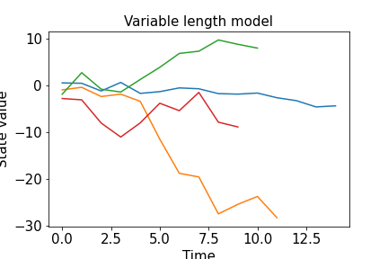
def var_length_ts_model(mean_timesteps=10):
    timesteps = pyro.sample(
        "timesteps",
        dist.Poisson(mean_timesteps)
    )
    dgp = stsb3.sts.RandomWalk(t1=int(timesteps), name="dgp")
    dgp.has_fast_mode = False
    obs_scale = pyro.param("obs_scale", torch.tensor(1.0))
    obs = pyro.sample(
        "obs",
        dist.Normal(dgp(), obs_scale)
    )
    return obs
This kind of model might be useful to infer the characteristic stopping time (here named timesteps) of a system.
Tracing the model a few times lets us confirm that it has an open-universe structure.
Trace #1
odict_keys(['_INPUT', 'timesteps', 'obs_scale', 'dgp-loc', 'dgp-scale', 'dgp-ic', 'dynamic/dgp-noise-1', 'dynamic/dgp-noise-2', 'dynamic/dgp-noise-3', 'dynamic/dgp-noise-4', 'dynamic/dgp-noise-5', 'dynamic/dgp-noise-6', 'dynamic/dgp-noise-7', 'dynamic/dgp-noise-8', 'dynamic/dgp-noise-9', 'dynamic/dgp-noise-10', 'dynamic/dgp-noise-11', 'dynamic/dgp-noise-12', 'dynamic/dgp-noise-13', 'dynamic/dgp-noise-14', 'dynamic/dgp-generated', 'obs', '_RETURN'])

Trace #2
odict_keys(['_INPUT', 'timesteps', 'obs_scale', 'dgp-loc', 'dgp-scale', 'dgp-ic', 'dynamic/dgp-noise-1', 'dynamic/dgp-noise-2', 'dynamic/dgp-noise-3', 'dynamic/dgp-noise-4', 'dynamic/dgp-noise-5', 'dynamic/dgp-noise-6', 'dynamic/dgp-noise-7', 'dynamic/dgp-noise-8', 'dynamic/dgp-noise-9', 'dynamic/dgp-noise-10', 'dynamic/dgp-noise-11', 'dynamic/dgp-generated', 'obs', '_RETURN'])

Trace #3
odict_keys(['_INPUT', 'timesteps', 'obs_scale', 'dgp-loc', 'dgp-scale', 'dgp-ic', 'dynamic/dgp-noise-1', 'dynamic/dgp-noise-2', 'dynamic/dgp-noise-3', 'dynamic/dgp-noise-4', 'dynamic/dgp-noise-5', 'dynamic/dgp-noise-6', 'dynamic/dgp-noise-7', 'dynamic/dgp-noise-8', 'dynamic/dgp-noise-9', 'dynamic/dgp-noise-10', 'dynamic/dgp-generated', 'obs', '_RETURN'])

Trace #4
odict_keys(['_INPUT', 'timesteps', 'obs_scale', 'dgp-loc', 'dgp-scale', 'dgp-ic', 'dynamic/dgp-noise-1', 'dynamic/dgp-noise-2', 'dynamic/dgp-noise-3', 'dynamic/dgp-noise-4', 'dynamic/dgp-noise-5', 'dynamic/dgp-noise-6', 'dynamic/dgp-noise-7', 'dynamic/dgp-noise-8', 'dynamic/dgp-noise-9', 'dynamic/dgp-generated', 'obs', '_RETURN'])
stsb3 is very opinionated about how you should construct structural time series models; the objective isn’t to be overly restrictive, but rather just restrictive enough that model complexity doesnt turn into model complication or model unwieldiness.
The first set of restrictions is associated with how stsb3 tracks randomness. In addition to all the wonderful low-level pyro machinery, stsb3 does its own tracing of randomness at the Block level. All addresses of block random variables follow a semantic naming convention that looks like either y-z or x/y-z.
y: the name of the block – this is what you’d pass into the constructor of the block via the keyword argument name=<your name here>.z: the functionality of the random variable. Examples include loc, scale, ic, seasons,…x: if it exists, this denotes special structural interpretation to the random variable. For example, dynamic denotes that there’s one of these kinds of random variables for each t in the interval [t0, t1].Thankfully, you usually don’t have to think about these addresses at all. Unless you’re writing your own Block subclass (discussed in the next section), all of these addresses will be automatically generated for you. Said differently, if you’re using any of the default blocks, you do not have any control over what the internal random variables are named.
This address structure simplifies a lot of reasoning about complex structural time series models. Here’s an important example. Suppose you’ve performed inference, and found an empirical posterior density of all model rvs – now it’s time to forecast. A posterior forecast is different from a draw from the posterior predictive; it’s equivalent to drawing values for all non-time-dependent random variables from the posterior and drawing values for all time-dependent variables from the fast-forwarded prior (i.e., the prior where t -> t + (t1 - t0)). This isn’t easy to do in an arbitrarily complex model, unless you have a semantic address structure like the one stsb3 implements. Then it’s as easy as checking if x = dynamic in the address structure, and if so, drawing from the fast-forwarded prior.
The z component of addresses aren’t any old string. Rather, they’re defined in stsb3.constants and are intended for cross-block use. They have semantic meaning; seeing z = loc tells you something about what the address my_block-loc is doing inside the block named my_block. Here are all of the currently-defined z components:
ic, obs, loc, scale, noise, dt, alpha, beta, plate, period, phase, amplitude,
lengthscale, seasons
You can add a new address component using core.register_address_component, with signature core.register_address_component(name, expand, domain=None). For example, calling
core.register_address_component(
    "my_component",
    True,
    domain=constants.real
)
adds a new z address component my_component that can be expanded into another block and whose domain is all real numbers. Currently defined domains are constants.real, constants.half_line (corresponding to the interval (0,oo)) and constants.zero_one. It’s necessary to state whether or not the address can be expanded into a block in order for structure search algorithms (still under development) to know if they can expand the site corresponding to this address. Most users will never interact with core.register_address_component because it’s only used when you’re defining a new block “by hand” rather than using the built-in block construction capabilities.
Valid stsb3 models are sentences in the language generated by the context-sensitive grammar G = (V, E, R, S), where V = {S, p}, E = {f, s}, and R consists of the production rules
S -> f(p) | f(p) + S
p -> s | (S | p, ..., S | p)
This means that valid models can be constructed by “adding” together functions of ps, by expanding ps into more models, or by letting ps become terminal nodes s, which for us are a random-variable-like objects (e.g., pyro.distributions objects or torch.Tensors, and probably in a later release pyro generative functions). “Adding” is in quotes because it doesn’t have to be the normal binary addition operation (although it usually is), but rather a symmetric group operation (like addition on real numbers or multiplication on positive reals). stsb3 doesn’t provide a static check to ensure that the model you’ve constructed is a valid sentence in the language generated by this grammar, but if you can call .model(...) on it and it doesn’t throw an error, then it’s a valid sentence.
An earlier version of this library (built using only numpy and scipy, and not recommended for production use) also included changepoints in the model grammar. This is no longer supported for two reasons. First, this necessarily makes the models non-generative. One of stsb3’s primary objectives is to ensure that all models have an explicit generative story and aren’t just some black-box stochastic process. Second, the task of forecasting seriously lowers the utility of a changepoint model, and one of stsb3’s other primary objectives is to enable white-box forecasting, not just modeling. It doesn’t make sense to talk about forecasting a changepoint model into the future; if you want a model that switches between different behaviors depending on a latent time series, then you just want a switching model. It’s easy to implement that yourself in stsb3 – we’ll demonstrate it in the next section.
If the existing set of building blocks isn’t enough for you, you can take two approaches: 1) you can pester us to implement more; 2) you can do it yourself. We recommend the latter choice. In this section we’ll outline different methods for implementing a Block or NoiseBlock subclass, and in the process detail more of stsb3’s internal structure.
All blocks inherit from stsb3.core.Block either directly or via stsb3.core.NoiseBlock. The only methods that a specific implementation must override are __init__ and _model. The heart of the specific implementation is _model, which describes the actual data generating process of the block. (This method isn’t called model because that’s a Block method that handles logic related to memoization and other internal interpretation details.) Here is the actual __init__ method for DiscreteSeasonal:
def __init__(
        self,
        name=None,
        t0=0,
        t1=2,
        size=1,
        n_seasons=2,
        seasons=None,
    ):
        super().__init__(
            name=name,
            t0=t0,
            t1=t1,
            size=size,
        )
        assert n_seasons >= 2
        self.n_seasons = n_seasons
        setattr(
            self,
            constants.seasons,
            seasons
            or dist.Normal(0.0, 1.0).expand(
                (
                    size,
                    n_seasons,
                )
            ),
        )
        self._maybe_add_blocks(getattr(self, constants.seasons))
The only things to note here are how we deal with the random object seasons. First, we have to respect stsb3’s naming conventions (well, okay, you don’t have to, but it’s highly recommended), so we setattr it using constants.seasons instead of the string "seasons". This way, if we later decided to change constants.seasons to some other string, that change would propagate to this implementation and we wouldn’t even notice. Second, we call _maybe_add_blocks on the newly-defined attribute with address component constants.seasons. This method checks to see if the attribute subclasses block. If it does, then the attribute is added to the block-level compute graph:
seasons = stsb3.sts.MA1(t1=t1, size=n, name="ma")
dgp = stsb3.sts.DiscreteSeasonal(
    t1=t1,
    size=n,
    name="s",
    n_seasons=len(seasons),
    seasons=seasons
)
stsb3.util.get_graph_from_root(dgp)

output$ {'s': ['ma'], 'ma': []}
Here’s DiscreteSeasonal’s _model method:
def _model(
        self,
    ):
        seasons = core._obj_name_to_definite(self, constants.seasons, season=True)
        t = torch.linspace(self.t0, self.t1, self.t1 - self.t0)
        which_seasons = torch.remainder(t, self.n_seasons)
        these_seasons = seasons[..., which_seasons.type(torch.LongTensor)]
        with autoname.scope(prefix=constants.dynamic):
            path = pyro.deterministic(
                f"{self.name}-{constants.generated}", these_seasons
            )
        return path
The actual functionality of this should be pretty clear. The only stsb3-specific aspects are
core._obj_name_to_definite to interpret what is meant by the object getattr(self, constants.seasons). The return value of this function, seasons, is just a torch.Tensor of shape (self.size, self.t1 - self.t0). How getattr(self, constants.seasons) becomes this tensor is decided by _obj_name_to_definite.pyro’s excellent contrib.autoname to ensure that all dynamic rvs (rvs whose last dimension is equal to self.t1 - self.t0) have x = dynamic in their address.So, to implement a new block, you could just subclass stsb3.core.Block and implement your own constructor and _model method. Or, you could try…
stsb3 doesn’t implement a random chirp model,and we really want one for our application. Because we’re lazy, we don’t want to actually write a class ourselves; we’d rather just implement a stochastic function in pyro and let stsb3 figure out the rest. Here’s how we’d do this:
Create a parameter dictionary. For a chirp model, that might look something like params = { "alpha": { "expand": True, "domain": constants.real, "default": dist.Normal(0.0, 1.0), }, "beta": { "expand": True, "domain": constants.real, "default": dist.Normal(0.0, 1.0), }, "gamma": { "expand": True, "domain": constants.real, "default": dist.Normal(0.0, 1.0), }, } Our chirp model will look like z_t = cos(alpha + beta * t + gamma * t ** 2).
Write a pyro function. This function has to take in some object (that we’ll creativey call x) that has appropriately-named attributes. In this case, the attributes will be named "alpha", "beta" and "gamma".
def chirp_model(x):
    alpha, beta, gamma = core.name_to_definite(x, "alpha", "beta", "gamma")

    with autoname.scope(prefix=constants.dynamic):
        t = torch.linspace(x.t0, x.t1, x.t1 - x.t0)
        path = pyro.deterministic(
            x.name + "-" + constants.generated,
            (alpha + t * beta + t.pow(2) * gamma).cos(),
        )
    return path
Make the block. We want the block to be named stsb3.sts.Chirp.
stsb3.sts.register_block(
    "Chirp",
    params,
    chirp_model,
)
That’s it. Now you can call and use this block as you would any other instance of a subclass of Block. See test_composition in test_sts.py for an example of this block in action.
Earlier we promised to implement a switching model. Let’s do that. The model itself is really simple – we’ll outsource the actual definition of the component time series x, y, and z to other blocks. The switching mechanism is defined in pseudocode thus:
for t in 1:T
    if x[t] < 0
        dgp[t] = y[t]
    else
        dgp[t] = z[t]
    end
end
Let’s see how to implement this using the block construction tools. First, we define the parameters of the block:
params = {
    "switch": {
        "expand": True,
        "domain": constants.real,
        "default": dist.Normal(0.0, 1.0)
    },
    "dgp1": {
        "expand": True,
        "domain": constants.real,
        "default": None
    },
    "dgp2": {
        "expand": True,
        "domain": constants.real,
        "default": None
    }
}
Then we implement the data generating process.
def switching_model(x):
    (switch,) = core.name_to_definite(x, "switch")
    mask = (switch < 0).type(torch.BoolTensor)
    with pyro.poutine.mask(mask=mask):
        (dgp1,) = core.name_to_definite(x, "dgp1")
    with pyro.poutine.mask(mask=~mask):
        (dgp2,) = core.name_to_definite(x, "dgp2")
    with autoname.scope(prefix=constants.dynamic):
        path = pyro.deterministic(
            x.name + "-" + constants.generated,
            torch.where(
                switch < 0,
                dgp1,
                dgp2
            )
        )
    return path
Finally, we construct the block and visualize some sample paths.
stsb3.sts.register_block("Switch", params, switching_model)
switch = stsb3.sts.AR1(t1=t1, size=n, name="switcher", beta=torch.tensor(0.75))
rw = stsb3.sts.RandomWalk(t1=t1, size=n, name="dgp1")
gt = stsb3.sts.GlobalTrend(t1=t1, size=n, name="dgp2")
switching_model = stsb3.sts.Switch(
    t1=t1,
    size=n,
    switch=switch,
    dgp1=rw,
    dgp2=gt,
)
We can comfort ourselves that all the desired pyro functionality is still there:
trace = pyro.poutine.trace(switching_model).get_trace()
assert trace.nodes["dgp1-" + constants.loc]["mask"] is not None